Intro to Machine Learning

Historical Background 02:55

AI Timelines

We live in very interesting times—nobody predicted this pace. A book from 2018 asked prominent researchers when human‑level AI might arrive; the closest answer was 2029, and most placed it fifty years away. Yet since late 2022, progress has only accelerated, with frontier labs now using their own models to make better models.

Early Thoughts on Artificial Intelligence 12:29

The idea of creating intelligence is ancient. In Greek myth, Hephaestus built androids: Talos, the bronze giant who guarded Crete by throwing rocks at enemy ships. What is interesting is how the difficulty of tasks reversed in reality: the Greeks already had accurate long‑range projectile weapons, but automatically recognising an enemy ship—a classic computer vision problem—proved far harder for humanity than the rock‑throwing part. Other traditions share similar themes: Pygmalion brought Galatea to life; in the Judean legend, wise rabbis created golems that could understand and obey but never speak, because speech was thought to require a soul. Today we know that speech synthesis is far easier than speech recognition—the exact opposite of the myth.

Mechanical Automata 17:57

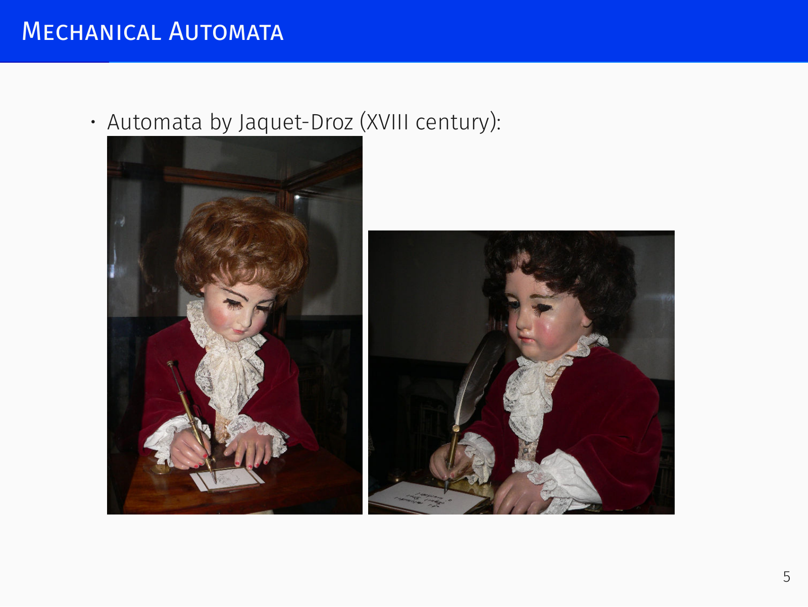
Early automata were inventive: al‑Jazari (12th century), the automata at Hesdin Castle, Leonardo’s mechanical knight. One of the most remarkable is Pierre Jaquet‑Droz’s 18th‑century calligrapher—a programmable doll that wrote different letters via a system of levers on its back. It was, to our knowledge, the first programmable device, predating Jacquard looms and punched cards. Still, it was purely mechanical; mathematical or logical intelligence remained rudimentary for centuries (Ramon Llull’s logical machine being a notable, though stretched, early effort).

The Turing Test 21:40

AI as a science began with Alan Turing’s 1950 paper “Computing Machinery and Intelligence.” The original test: a judge chats in writing with two hidden entities—a human and a computer—and must distinguish them. A single run means nothing; the program passes only when, over many trials, the judge cannot distinguish it from a human with probability different from ½. This immediately places the test in the realm of probability theory and randomised algorithms.

The Turing test survived longer than almost any other AI benchmark. It was formally passed only in 2025, after models like GPT‑4 could be made to stay in character and fool judges in extended conversations. This is remarkable because AI has a long history of moving goalposts: when Deep Blue beat Kasparov, chess was dismissed as “just tree search”; when AlphaGo mastered Go, the bar shifted again. The Turing test resisted because it hinges on free‑form natural language. A judge can ask anything—demand a drawing, describe a 3D scene, request a joke about a specific topic. To maintain consistency, the other side must understand the physical world and a vast range of human knowledge. Natural language is complete in this sense, which is precisely why large language models are so powerful: to predict the next token well they must internalise an enormous amount of world structure (robotics being a notable exception, as we lack large text corpora describing low‑level motor actions).

The test is also fundamentally unfair to computers: in a reverse Turing test, a human would fail immediately because a 1950s computer could instantly compute $37^{23}$. The original essay even included a detail about gender impersonation that has often been forgotten. But it got people thinking about what intelligence requires.

The Dartmouth Workshop and the Birth of AI 41:11

AI as a field was born in 1956 at the Dartmouth workshop, organised by John McCarthy, Marvin Minsky, Claude Shannon, and Nathaniel Rochester. The grant proposal is probably the most ambitious in computing history:

We propose a 2-month study of artificial intelligence to be carried out by 10 people in the summer of 1956 … The study is based on the conjecture that every aspect of learning or any other feature of intelligence can in principle be so precisely described that a machine can simulate it. We will attempt to find how to make machines use natural languages, form abstractions and concepts, solve problems now reserved for humans, and improve themselves.

The workshop took place, but they did not solve these problems—they mainly began to grasp how difficult they were.

1956–1960: High Expectations 43:05

Optimism ran high. The Logic Theorist successfully re‑proved most of Principia Mathematica, sometimes more elegantly than Russell and Whitehead, fuelling the belief that teaching AI logic and mathematics was the key. The General Problem Solver tried to think like a human. Many specialised programs operated in microworlds: Analogy solved IQ tests, Student handled algebraic word problems, and Blocks World simulated 3D block manipulation.

1970s: Knowledge‑Based Systems 46:06

The 1960s ended with disappointment, especially after the failure of machine‑translation projects, leading to the “AI winter.” The only active branch was expert systems. The prime example is MYCIN, a medical diagnosis system for blood infections. A blood test produces about 50 numbers; a physician uses local heuristics like “if red blood cell count is high and iron is low, then disease X.” The challenge is that terms like “high” are fuzzy and many rules partially apply. MYCIN had about 450 rules and performed as well as experienced physicians, significantly better than novices.

1980s: Commercial AI and the Next Winter

The first AI department at DEC reportedly saved the company around $10 million annually by 1986. The boom ended in the late 80s when many companies failed to meet inflated expectations.

1990–2010: Data Mining, Machine Learning 49:35

The focus shifted to learning from data, accelerated by the growth of the Internet. Early neural networks—convolutional, recurrent, deep—existed conceptually but lacked data and compute. The deep‑learning revolution took off in the mid‑2000s, when labs (notably Geoffrey Hinton’s and Yoshua Bengio’s) had enough internet‑scale data and computational power, especially through GPUs with their thousands of cores that make the parallelisable operations of neural nets feasible. Deep learning has set the state of the art in many fields since the late 2000s, culminating in the LLM revolution—a very different, ongoing story.

What is Machine Learning? 52:26

A computer program learns from experience $E$ with respect to a class of tasks $T$ and a performance measure $P$, if its performance on tasks in $T$ (measured by $P$) improves with experience $E$.

The definition sounds trivial, but the key is having a number that goes up or down. In a sense, half of deep learning is inventing loss functions—deciding what number we want to minimise so that minimising it yields the behaviour we actually want.

Key ML Tasks and Concepts 54:15

Supervised Learning

• Learning from a set of labelled examples. Each example consists of features $X$ and a correct answer $Y$, the response variable we want to predict (categorical, continuous, or ordinal).
• The model learns a function $f(X)$ meant to match $Y$. Mathematically, we aim to learn the conditional distribution $p(y \mid x)$; the input is given and the output is relatively simple compared to the often high‑dimensional input.
• The main goal is generalisation to new examples; otherwise we have overfitting. We check generalisation via cross‑validation: splitting data into training and validation sets.
• Preprocessing and feature extraction often precede modelling.
• Two main tasks:
  • Classification: assign to a discrete class. E.g., text classification by topic, spam filtering, face/object/text recognition.
  • Regression: predict the value of an unknown function. E.g., engineering predictions (temperature, robot position), stock prices, speech recognition.

Collecting labels, especially for tasks like image segmentation, is often extremely expensive, so we work with relatively small labelled datasets.

Unsupervised Learning 59:53

Learning without labels—only raw data. Common tasks:

• Clustering: partition data into unknown groups based on similarity (e.g., gene families, user personalisation).
• Dimensionality reduction: data has huge dimensionality and we need to select the most informative features (representation learning). An image of 1 megapixel with 3 colour channels is a point in a space of about 3 million dimensions. The set of real images is a very complicated manifold; unsupervised learning tries to compress this manifold to a manageable size (say 500) while preserving the ability to answer interesting questions. In the compressed space, cats and dogs might become linearly separable.
• Matrix completion: predict missing entries in a sparse matrix.

A natural framework is the autoencoder: an encoder network compresses $x$ to a low‑dimensional code $z$, a decoder network tries to reconstruct $\hat{x}$ from $z$. The loss is simply the reconstruction error, e.g. $(\hat{x} - x)^2$. The model learns to encode information that matters for reconstruction. Clustering can be viewed as an extreme case—compressing each point to a discrete label (zero‑dimensional code) and then reconstructing by the cluster centre.

Whereas supervised learning models $p(y \mid x)$, unsupervised learning models $p(x)$ itself, often yielding generative models that can produce new samples from the data distribution.

Reinforcement Learning 1:17:06

An agent learns from its own trial‑and‑error interactions with an environment. Fundamental challenges:

• Multi‑armed bandits: choosing actions that lead to random rewards, maximising cumulative reward.
• Exploration vs. exploitation: when to try new actions vs. stick with known good ones.
• Credit assignment: reward is often delayed (e.g., winning a game); we must assign credit to each individual action that led to success.

This course does not cover reinforcement learning.

Other Learning Paradigms

• Active learning – choosing the next (usually expensive) test to label.
• Learning to rank – producing ordered lists (e.g., internet search results).
• Bootstrapping – using a model’s own outputs to improve itself.
• Model selection – balancing models with few vs. many parameters.

Probability in Machine Learning 1:45:08

Methods that not only give an answer but also estimate confidence, describe data quality, and anticipate changes with further experiments rely on probability theory. Fortunately, we only need the standard intuition of discrete and continuous random variables—no measure theory, sigma‑algebras, or exotic spaces. The probability spaces we work with are Euclidean spaces $\mathbb{R}^d$ with a density.

Bayesian Approach to Machine Learning 1:57:11

Basic Probability Definitions

• Joint probability: $p(x, y)$, probability of two events simultaneously.
• Marginalisation: $p(x) = \sum_y p(x, y)$ (or integral for continuous).
• Conditional probability: $p(x \mid y) = \frac{p(x, y)}{p(y)}$ (provided $p(y) > 0$).
• Bayes’ theorem:
  $$p(y \mid x) = \frac{p(x \mid y)\, p(y)}{p(x)} = \frac{p(x \mid y)\, p(y)}{\sum_{y'} p(x \mid y')\, p(y')}.$$
• Independence: $x$ and $y$ are independent if $p(x, y) = p(x)\, p(y)$; then $p(x \mid y) = p(x)$.

Bayesian Inference for Parameters

For parameter estimation, Bayes’ theorem reads:

• $p(\theta)$ — the prior distribution (what we believed about $\theta$ before seeing data).
• $p(D \mid \theta)$ — the likelihood (probability/density of the observed dataset given the parameters).
• $p(\theta \mid D)$ — the posterior distribution (our updated belief after data).
• $p(D) = \int p(D \mid \theta)\, p(\theta)\, \mathrm{d}\theta$ — the evidence (a normalising constant, usually inaccessible).

Because $p(D)$ does not involve $\theta$, we often work with the proportionality

Maximum Likelihood vs. Maximum a Posteriori

Two point estimates are common in practice:

• Maximum likelihood (ML):
  $$\theta_{\text{ML}} = \arg\max_\theta p(D \mid \theta).$$
• Maximum a posteriori (MAP):
  $$\theta_{\text{MAP}} = \arg\max_\theta p(\theta \mid D) = \arg\max_\theta p(D \mid \theta)\, p(\theta).$$

The logarithm of the posterior is $\log p(D \mid \theta) + \log p(\theta) + \text{constant}$. In optimisation, $\log p(\theta)$ acts as a regulariser—it incorporates our prior beliefs about the parameters, penalising values that are unlikely a priori. This is a direct bridge from Bayesian inference to deep learning regularisation.

Direct and Inverse Problems

• Direct problem: given a probabilistic model, predict behaviour. E.g., an urn has 10 balls, 3 black; what is the probability of drawing a black ball?
• Inverse problem: observe behaviour and infer hidden parameters. E.g., an urn is known to have either 3 or 6 black balls; you draw a black ball; what is the probability it was the first urn?

Machine learning problems are almost always inverse: we observe data and must build a probabilistic model of the hidden variables that generated it.

Probability as Frequency vs. Degree of Belief

Classical probability interprets probability as the limit of relative frequencies over repeated experiments (e.g., coin tosses). But we often want to reason about events like “Spain wins the 2026 World Cup” or “the Odyssey was written by a woman”—unique events where infinite repetitions are meaningless. In such cases, probability becomes a degree of belief. This is the Bayesian interpretation, and it follows the same mathematical laws as frequency‑based probability.

Examples

1. Two children problem A person has two kids; each is equally likely a boy or a girl.

   • (1) “Do you have any boys?” “Yes.” Probability of also having a girl?
   • (2) “I met one of your kids, and it’s a boy.” Probability the other is a girl?

2. Prosecutor’s fallacy A rare blood type (1 % prevalence) is found at a crime scene and matches the defendant.

   • (1) Prosecutor: “There is only a 1 % chance of a match if innocent, so with 99 % probability he is guilty.” Mistake: the probability of guilt is not $1 - p(\text{match} \mid \text{innocence})$; it requires the prior probability of guilt and all alternative suspects.
   • (2) Defense: “A million people live in the city, so 10000 have this blood type. The blood only gives a 0.01 % probability of guilt.” Mistake: all those 10000 people together still only account for a small fraction of the city; the evidence is not worthless.

3. Real cases The O.J. Simpson trial and the Sally Clark case (two SIDS deaths) both involved mis‑applied probability—the court sometimes confused conditional probabilities and ignored base rates.

Bayesian Inference for a Coin 2:05:13

Problem Statement

We have an unfair coin with (unknown) probability $p_h = \theta$ of heads. Flipping it $N$ times yields a sequence $s$ with $n$ heads and $m$ tails. Assuming flips are independent given $\theta$, the likelihood is

In machine learning, defining the model means writing down this likelihood—specifying the assumptions (mutually exclusive outcomes, conditional independence) that let us produce the formula. This is the easy part.

Maximum Likelihood and Its Pitfalls

Maximising the likelihood directly gives $\theta_{\text{ML}} = \frac{n}{n+m}$. For a coin with many tosses, this matches the frequency limit and is correct.

But suppose we toss the coin once and get tails. The likelihood is $1 - \theta$. Without constraints it would be maximised at $-\infty$; with the constraint $0 \le \theta \le 1$, the maximum likelihood estimate is $\theta = 0$—we would claim the coin always lands tails. After a single toss, that conclusion is absurd. The maths is correct, but the estimate is unreliable because we have almost no data.

In real machine learning, data is almost always insufficient. When you finally have enough data for your current model, it is often better to move to a larger model (e.g., from GPT‑1 to GPT‑2) for which you are again data‑limited. We constantly operate at the frontier where data is scarce. So a point estimate based on the likelihood alone is rarely enough. We need to bring in our prior beliefs.

Introducing the Prior

Bayes’ rule gives the posterior

The prior $p(\theta)$ represents what we believed about $\theta$ before seeing the data. For a coin, the most basic reasonable belief is that $\theta$ must lie in $[0,1]$, so $p(\theta) = 0$ outside that interval. A common uninformative choice is a uniform prior $p(\theta) = 1$ for $\theta \in [0,1]$, expressing complete ignorance. With $n$ heads and $m$ tails, the posterior becomes

The denominator is a Beta integral, $B(n+1, m+1) = \frac{n!\, m!}{(n+m+1)!}$, but for point estimation we only need the proportionality.

Posterior Distribution and MAP

Maximising the posterior with a uniform prior yields the same estimate as maximum likelihood: $\theta_{\text{MAP}} = \frac{n}{n+m}$. The prior only rules out degenerate solutions ($\theta=0$ or $\theta=1$ with a single observation would give a posterior of 0), but the location of the maximum is unchanged. So MAP with a uniform prior does not fix the overconfidence of the point estimate when data is scarce.

Predictive Distribution and Laplace’s Rule

The ultimate goal is not the parameter $\theta$ but prediction. Given past data, we want the probability of the next outcome, $p(\text{heads} \mid s)$. This quantity does not depend on $\theta$; it is obtained by averaging the likelihood over the posterior:

Evaluating the integral gives Laplace’s rule of succession:

Even with a uniform prior, the predictive distribution is different from the point estimate $\frac{n}{n+m}$. For example, after one tail ($n=0, m=1$) the point estimate says $0$, but Laplace’s rule says $\frac{1}{3}$—a much more reasonable belief. As data accumulates, the two converge, but with little data the advantage of averaging over the whole posterior is decisive.

This illustrates the two main Bayesian tasks:

1. Find the posterior $p(\theta \mid D) \propto p(D \mid \theta)\, p(\theta)$ and/or the MAP hypothesis.
2. Find the predictive distribution for future observations: $p(x \mid D) = \int p(x \mid \theta)\, p(\theta \mid D)\, \mathrm{d}\theta$.

The predictive distribution is the expectation over the posterior of the likelihood, and it is almost always what we want from a machine learning system. In neural networks, $\theta$ are the weights; we care about predictions on new images, not the weights themselves. The Bayesian framework makes this natural.

The Role of the Prior in Practice

When data is limited, the prior heavily influences the conclusion. A more realistic prior for a physical coin might be a bell‑shaped curve centred near $\frac{1}{2}$ (e.g., a truncated normal). But multiplying such a prior by the polynomial likelihood $\theta^n (1-\theta)^m$ yields an expression that is not a standard distribution—tractable only numerically. Since our intuition does not specify the exact shape of the bell, we are free to choose a prior that is mathematically convenient, provided it captures the rough features (bounded between 0 and 1, peak near $\frac{1}{2}$). This leads directly to the idea of conjugate priors.

Conjugate Priors 3:05:58

Prior Distributions

In Bayesian inference, after choosing the likelihood we must also choose a prior $p(\theta)$. The prior is a distribution over all possible parameter values, and its shape strongly affects the results, especially with small datasets. To simplify computation, we want the posterior $p(\theta \mid x)$ to belong to the same parametric family as the prior $p(\theta)$. If this holds, we can update hyperparameters directly without new integrals.

Conjugate Priors

A family of distributions $p(\theta \mid \alpha)$ is a conjugate prior for a family of likelihoods $p(x \mid \theta)$ if, after multiplying by the likelihood, the posterior stays in the same family: $p(\theta \mid x, \alpha) = p(\theta \mid \alpha')$. The $\alpha$ are called hyperparameters — the parameters of the distribution of the parameters.

The trivial family of all distributions is conjugate, but that is not useful. The form of a useful conjugate prior depends on the form of the data likelihood.

Bernoulli Trials (Beta Prior)

For Bernoulli (coin‑toss) trials, the likelihood is proportional to $\theta^s (1-\theta)^f$ with $s$ successes and $f$ failures. The conjugate prior is the Beta distribution:

where $B(\alpha, \beta) = \frac{\Gamma(\alpha)\Gamma(\beta)}{\Gamma(\alpha+\beta)}$ is the beta function.

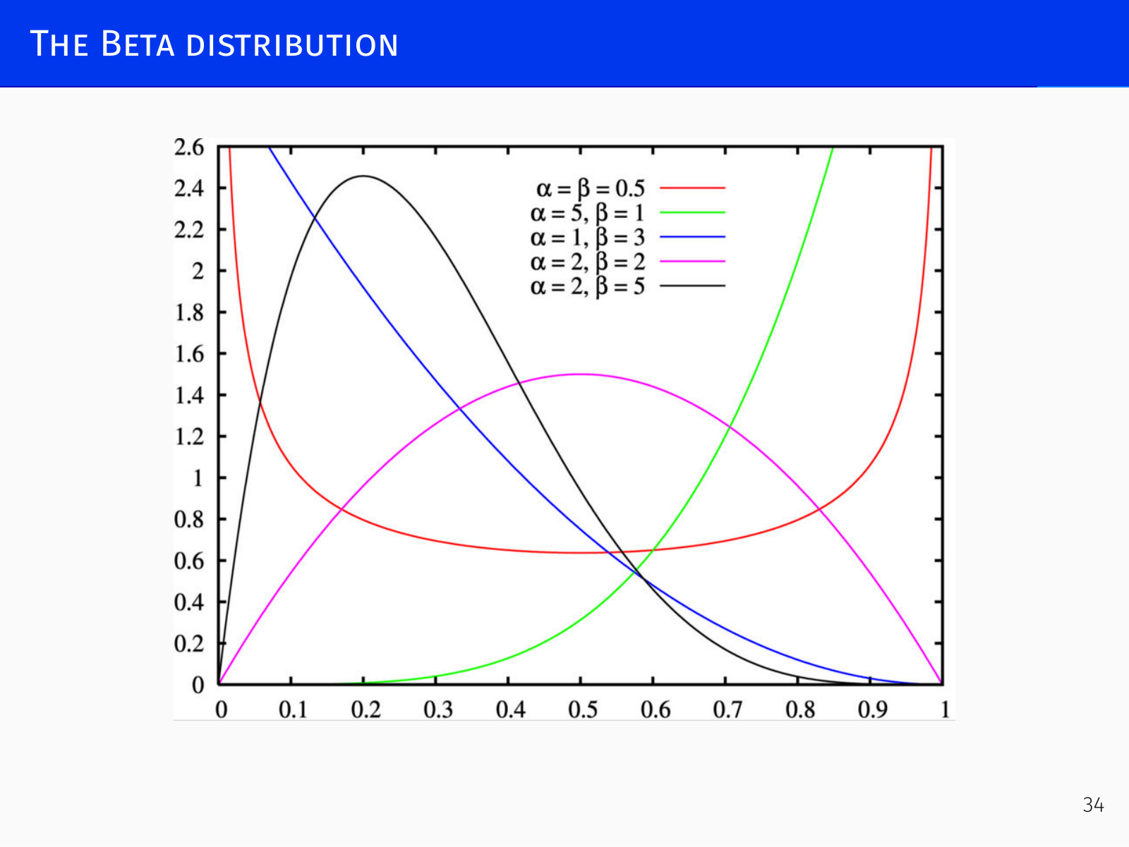
After observing $s$ heads and $f$ tails, the posterior is

which is again a Beta distribution, $\text{Beta}(s+\alpha, \, f+\beta)$. The learning rule is extremely simple: add the counts to the hyperparameters:

You can forget the complicated formulas. The hyperparameters $\alpha$ and $\beta$ can be interpreted as pseudo‑counts—fictitious prior observations. The uniform prior corresponds to $\alpha = \beta = 1$ ($\text{Beta}(1,1)$). A prior peaked around $\frac{1}{2}$ is obtained by setting, say, $\alpha = \beta = 10$; this encodes the belief that we have already seen (virtually) 10 heads and 10 tails, and it takes a substantial amount of real data to shift the posterior away from $\frac{1}{2}$.

Because the posterior has the same form as the prior, Bayesian updating can be done sequentially: start with a prior, incorporate a data batch, obtain a posterior, then treat that posterior as the new prior for the next batch. This avoids reprocessing all data from scratch.

The predictive distribution for a new trial, using a Beta $(\alpha, \beta)$ prior, generalises Laplace’s rule:

Multinomial Distribution (Dirichlet Prior)

A natural extension is rolling a die with $k$ faces, modelled by a multinomial distribution. If $x_i$ observations fall into category $i$, the likelihood is

The conjugate prior is the Dirichlet distribution:

After observing counts $x_1, \dots, x_k$, the hyperparameters update analogously:

This simplicity of updating makes conjugate priors a cornerstone of tractable Bayesian inference.