Convolutional Architectures and Beyond

Weight Reuse, Classical Filters, and Visualizing Learned Filters 00:16

The defining advantage of convolutional neural networks is weight reuse: the same filters are applied across the entire input and over all intermediate feature tensors, dramatically reducing the number of parameters while enabling massive parallelism.

Before deep learning, convolutions were used as handcrafted filters in classical computer vision. Small matrices were slid over an image to perform operations such as sharpening, blurring, embossing, or edge detection. For instance, Gabor filters compute discrete directional derivatives – one filter fires on large vertical differences between adjacent pixels, another on horizontal changes. Applying max pooling as an image filter would simply clamp to maximum brightness (producing unnatural results), while average pooling appears smoother but is not meant to be a pixel-level transformation.

In a real network like ResNet-18, the first layer’s convolutional filters can be inspected. Some detect diagonal or vertical lines, others respond to colors or colour gradients. When an input image is passed through, one filter might fire where green appears (grass/trees), another for horizontal edges. Deeper in the network, direct pixel‑to‑feature correspondence disappears – each unit has a receptive field, but tracing exactly which pixels contribute requires additional mathematics. Nevertheless, one can observe what upper‑layer features respond to. In ResNet-18, the second layer activates on high‑frequency content (stripes, edges) across the whole image. Deeper layers respond to more semantic structures: a filter might detect eyes and ear tips, and even deeper ones fire on entire heads. Visualizations become progressively blurrier and less geometric, but the features can be mapped back to the original image to approximate what triggers them.

At a late layer, features can be strongly class‑selective. A cat‑selective feature correlates strongly with the “cat” class on ImageNet. If you present a composite image half‑cat, half‑dog, the cat‑selective feature fires on the cat half and a dog‑selective feature fires on the dog half, demonstrating genuine selectivity.

A more detailed explanation method is GradCAM. Given a classification network, running GradCAM on a specific class output reveals which pixels contributed most to that output value. For example, the “Egyptian cat” logit responds because of certain image regions, while the “Blenheim Spaniel” logit focuses on other regions. This is not an attention mechanism; it provides a post‑hoc explanation of the network’s decision.

Important Convolutional Architectures

AlexNet 12:18

AlexNet (Krizhevsky, Sutskever, Hinton, 2012) was the architecture that kick‑started modern deep learning for computer vision. It dominated the ImageNet Large‑Scale Visual Recognition Competition by an extraordinary margin: competing methods had error rates around 22–23%, while AlexNet achieved ~13%. The following year the entire leaderboard switched to convolutional networks, and classical computer vision was abandoned for image classification.

Two key technical ideas made AlexNet possible:

Model parallelism was used for the first time at an industrial scale. The network was split into two parallel streams, each running on a separate GPU. Data parallelism, by contrast, simply splits a mini‑batch across GPUs, processes them in parallel, and then aggregates the gradients for a single update – the network implementation does not change. Model parallelism is necessary when the model does not fit on a single GPU. AlexNet was hand‑engineered by Alex Krizhevsky to explicitly assign layers to different GPUs while minimising cross‑GPU communication, which is slower than on‑chip communication. In modern frameworks such as PyTorch, specific weight matrices can be assigned to specific GPUs and communication is handled automatically.

VGG 17:31

VGG (Oxford Visual Geometry Group) represents large convolutions as compositions of smaller ones, typically stacks of $3 \times 3$ convolutions.

Using a stack of $3 \times 3$ filters reduces the number of weights compared to one large filter and makes the network deeper. It also acts as additional structural regularisation because the network processes different parts of the input in the same way.

VGG was used in the ILSVRC‑2014 competition, and NVIDIA later optimised GPUs especially for $3 \times 3$ convolutions. The idea of treating a large convolution as a “convolution inside a convolution” proved very effective.

Inception (GoogLeNet) 19:12

The Inception architecture and its realisation in GoogLeNet employ the “network in network” concept to reduce the number of weights even further. Instead of using a single linear convolution over a tile, Inception units implement a more complex mini‑network that is still applied identically across all spatial positions. Another idea is to insert additional classifiers (and corresponding auxiliary loss terms) at intermediate layers of the network.

Inception units frequently feature multiple parallel processing branches, which is a deliberate design choice that will be explored in detail later.

Inception v2 and v3

In Inception v2 (Szegedy et al., 2015), $n \times n$ convolutions are replaced by $n \times 1$ followed by $1 \times n$ convolutions. Filter banks become wider rather than deeper. The same paper introduced Inception v3, which adds RMSProp optimisation, factorised $7 \times 7$ convolutions, batch normalisation in the auxiliary classifiers, and label smoothing.

Label Smoothing

A regular classifier trains the softmax with a hard target

Label smoothing replaces the hard target with a soft target:

$$q'(k) = (1 - \epsilon)[k = y] + \epsilon\, u(k)$$

where $u(k)$ is a prior distribution, often the uniform distribution $u(k) = \frac{1}{K}$. This prevents the network from becoming too certain and improves generalisation.

ResNet 21:46

Residual learning addresses the vanishing gradient problem by training differences rather than the full mapping.

A residual unit computes

$$y^{(k)} = F(x^{(k)}) + x^{(k)},$$

where $x^{(k)}$ is the input to layer $k$, $F$ is the function learned by the layer, and $y^{(k)}$ becomes $x^{(k+1)}$. The gradient can flow directly through the identity path:

$$\frac{\partial y^{(k)}}{\partial x^{(k)}} = 1 + \frac{\partial F(x^{(k)})}{\partial x^{(k)}},$$

so gradients do not vanish when $F$ saturates.

When a layer’s output $F(x)$ saturates and its derivatives approach zero, without a skip connection all layers below would stop receiving gradients. The identity shortcut guarantees a path for gradient flow, enabling extremely deep networks. Kaiming He introduced ResNets and called it the revolution of depth: AlexNet had 8 trainable layers, VGG 19, GoogLeNet 22, while ResNet immediately scaled to 150 layers, and networks of 200, 500, or even 1000 layers became trainable (practical ResNets typically go up to about 200 layers).

A related approach is highway networks (Schmidhuber), where the output is a gated combination:

$$y^{(k)} = C(x^{(k)})\,x^{(k)} + T(x^{(k)})\,F(x^{(k)}),$$

with $C$ a carry gate and $T$ a transform gate, usually satisfying $C = 1 - T$. In practice, residual connections work best when they are as “straight” as possible.

Bottleneck Layers and the Split-Transform-Merge Paradigm 25:44

Beyond the weight reduction achieved by VGG‑style small filters, an even more aggressive parameter saving is possible via bottleneck layers. Consider a standard convolutional layer operating on a cut‑out window of depth $D$, width $W$, height $H$, producing an output of depth $D'$. The weight tensor size is $D \times W \times H \times D'$. Even with small filters ($W = H = 3$) and moderate depths ($D = D' = 256$), this gives $256 \times 3 \times 3 \times 256 \approx 590\text{k}$ parameters.

A bottleneck first compresses the input channel depth with a $1 \times 1$ convolution to a much smaller dimension $D''$, then applies the spatial convolution, and finally expands back to $D'$ with another $1 \times 1$ convolution. If $D = 256$, $D'' = 32$ and $D' = 256$, the parameter count becomes

However, compressing a 256‑dimensional feature vector down to 32 numbers and then decompressing back to 256 cannot restore lost information. A single bottleneck branch would be senseless – one could simply let the previous layer produce 32 features instead and save even more weights. The bottleneck idea becomes powerful when multiple parallel branches are used. By creating several copies of the bottleneck block, each with its own independently learned weights, and concatenating their outputs, the network learns multiple low‑dimensional projections – different “viewpoints” – of the same high‑dimensional space, each capturing a different aspect of the data.

With $D = 256$, $D'' = 32$, and 8 branches, the total parameter cost is about $8 \times 25.6\text{k} \approx 205\text{k}$, compared to the original $590\text{k}$ – a 3–4‑fold saving. Geometrically, taking many (learned) random projections of a high‑dimensional object is often beneficial, and here the projections are trained to be useful. This approach is called split‑transform‑merge: split the input, transform each part, then merge the results. It is a standard pattern in convolutional architectures.

ResNeXt

ResNeXt (Xie et al., 2016) replaces ResNet units with “split‑transform‑merge” units reminiscent of Inception. The input channels are divided into groups, and every group receives its own convolutions. This is akin to group convolutions, already used in AlexNet for parallelisation, and yields a kind of specialisation in the resulting feature maps.

Inception v4 and Inception‑ResNet 42:41

Another classic paper (Szegedy et al., 2016) introduced Inception v4 and Inception‑ResNet. The Inception family long served as excellent backbones for many computer vision tasks: when labelled data is scarce, the standard practice is to take a model pretrained on ImageNet for classification, cut off its classification head, and use the rest as a feature extractor, possibly with light fine‑tuning.

• Inception v4 standardises everything and simplifies the units. A “stem” module is defined first, followed by three basic blocks (A, B, C) and special reduction blocks to reduce spatial dimensions. Instead of a fixed pooling operation, these reduction blocks are learnable compositions of layers with strided convolutions, often containing pooling internally and following the split‑transform‑merge pattern.
• Inception‑ResNet adds residual connections to these Inception blocks. There is no pooling, but reduction blocks are still employed, making the architecture even simpler. Inception‑ResNet v2 is a refined version that performs extremely well in practice and was one of the most widely used backbones around 2016.

SqueezeNet and MobileNet 46:52

When deploying networks, two resources must be balanced: memory (number of weights) and latency (number of sequential layers). GPU parallelism means that the number of layers often dictates latency more than the raw parameter count, though intermediate representation sizes also matter. Real‑time applications, such as surveillance tracking, require at least 30–60 frames per second, driving the need for extremely efficient architectures.

SqueezeNet (Iandola et al., 2017) aims to drastically reduce the number of parameters by:

• replacing $3 \times 3$ filters with $1 \times 1$;
• reducing the number of input channels for the remaining $3 \times 3$ convolutions;
• delaying downsampling as late as possible to keep activation maps large.

The core building block is the fire module, composed of a squeeze layer (only $1 \times 1$ convolutions) followed by an expand layer (a mix of $1 \times 1$ and $3 \times 3$ convolutions). This yields about 50× fewer parameters than AlexNet, at the cost of some accuracy.

MobileNet (Howard et al., 2017) designs networks specifically for mobile devices. It uses depthwise separable convolutions: a standard convolution is decomposed into a depthwise convolution (one filter per input channel) followed by a $1 \times 1$ convolution. This structure is more complex but has far fewer weights, and the overall architecture is not very deep. The approach saves many parameters with a small drop in quality.

EfficientNet 50:20

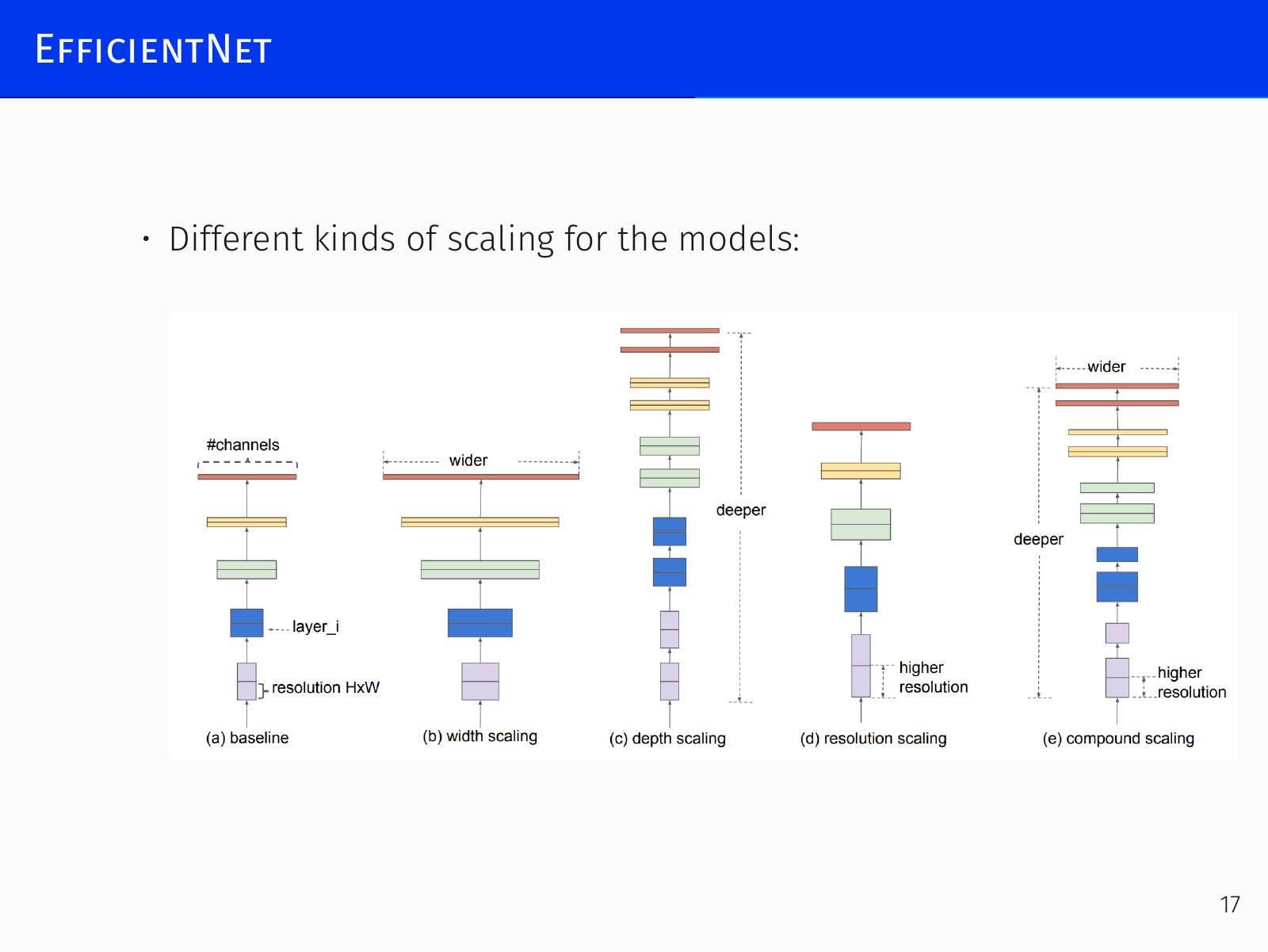
EfficientNet (Tan, Le, 2019) applies neural architecture search to find state‑of‑the‑art networks. The key insight is compound scaling: simultaneously scaling network depth, width, and input resolution yields better performance than scaling a single dimension. The search considers exponential scaling with exponents $\alpha$ (depth), $\beta$ (width) and $\gamma$ (resolution); the total number of weights scales as the product of these factors.

The efficiency landscape is often displayed on a plot with number of parameters on the x‑axis (fewer is better) and ImageNet top‑1 accuracy on the y‑axis (higher is better). The Pareto frontier connects the best possible network for every size, and for every target quality the smallest possible network. The EfficientNet family succeeded in defining this frontier, and it remains the best underlying convolutional backbone, widely used in object detection and segmentation pipelines.

Batch Normalization 56:14

The Internal Covariate Shift Problem

As weights of a layer change during training, the distribution of its outputs shifts. The next layer must then continually re‑adapt, and neurons that have reached saturation slow down retraining. This phenomenon – internal covariate shift – seriously impedes deep network training.

Why Naïve Solutions Fail

• Whitening after every layer: Consider a layer that adds a bias $b$ to its input $u$, producing $x = u + b$. If we normalise by subtracting the mean, $\hat{x} = x - \mathbb{E}[x]$, and then update $b := b + \Delta b$, the normalised output does not change:
  $$u + b + \Delta b - \mathbb{E}[u + b + \Delta b] = u + b - \mathbb{E}[u + b].$$
  The biases grow without bound while the normalised output remains unchanged, so training fails.
• Normalisation as a layer: $\hat{x} = \text{Norm}(x, X)$ requires the entire dataset $X$ to compute gradients $\frac{\partial \text{Norm}}{\partial x}$, $\frac{\partial \text{Norm}}{\partial X}$, as well as the full covariance matrix $\text{Cov}[x] = \mathbb{E}_{x \in X}[xx^\top] - \mathbb{E}[x]\mathbb{E}[x]^\top$, which is computationally prohibitive.

Batch Normalization (BN)

The solution is to normalise each feature component separately not over the whole dataset but over the current mini‑batch – hence batch normalisation. For a component $x_k$,

However, this forces the activations into the linear regime of nonlinearities (e.g., the sigmoid), which can destroy the network’s capacity. To remedy this, learnable shift and scale parameters are introduced:

What BN Actually Does

Although originally motivated by reducing internal covariate shift, subsequent research showed that BN’s effectiveness does not really depend on this. BN nevertheless provides regularisation, makes dropout often unnecessary, and significantly improves training. Possible explanations include:

• BN smooths the gradients, reducing the Lipschitz constant (Santurkar et al., 2019).
• BN decouples the learning of the direction and length of weight vectors, which improves training dynamics.
• There are results showing that BN helps achieve linear convergence in ordinary gradient descent.

Variants of Normalization

Many normalisation methods share the same general operations: compute statistics over some set, normalise, then apply a learned scale and shift. They differ in which dimensions the statistics are computed over.

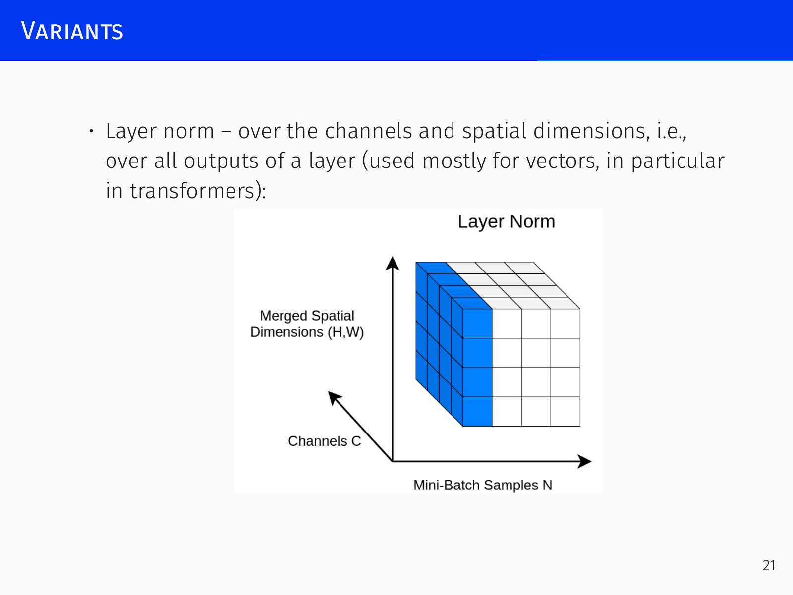
General form: compute mean and variance over a specified set of axes, normalise, then transform with $\gamma$ and $\beta$.

• Batch Normalization – over the mini‑batch dimension ($N$). Commonly used for images. It averages the same feature over spatial dimensions and across the mini‑batch.
• Layer Normalization – over all channels and spatial dimensions of a layer (all features of a single sample). Used mostly for vectors, in particular in transformers. Unlike batch norm, it does not average over the mini‑batch. In practice, when using layer norm the mini‑batch size is often one, so no mini‑batch statistics are available – you normalise over the whole tensor of features for one sample. This is essential for transformers, where large models rarely allow large mini‑batches.
• Instance Normalization – over the spatial dimensions ($H, W$) only, separately per sample and per channel. Used, e.g., in AdaIN for style transfer.
• Group Normalization – splits channels into groups and normalises over each group together with the spatial dimensions.
• Weight Standardization – instead of normalising activations, standardises the weights (per output channel). This effectively normalises the gradients during backpropagation. Group norm combined with weight standardisation was used in BiT (Big Transfer).

Further developments: Batch normalisation is not effective for recurrent networks (Laurent et al., 2016); recurrent batch normalisation was proposed (Cooijmans et al., 2016). Weight normalisation (Salimans and Kingma, 2016) re‑parameterises the weight vector as

Working with Sequences 58:19

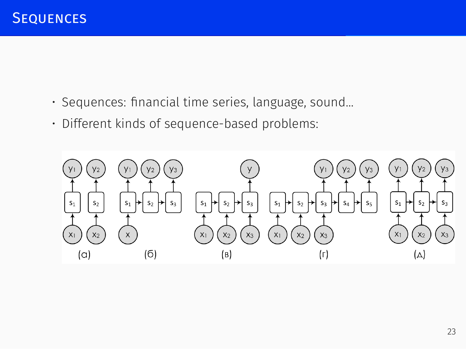
Many problems involve sequential data: financial time series, sound, or text. Unlike images, which are two‑dimensional structures naturally suited to CNNs, sequences are inherently one‑dimensional.

Several problem types exist:

• Sequence → single output: e.g., text classification – an entire news article is mapped to one category (sports, politics, science).
• Single input → sequence: e.g., image captioning – a still image is converted into a variable‑length text description.
• Sequence → sequence: e.g., machine translation – both input and output are sequences of variable length.
• Sequence labelling: the output is a label for each input element, aligned with the input. Examples include part‑of‑speech tagging (a label for every word), video subtitle addition (each frame gets a text), and object tracking (segmenting an object consistently across video frames).

A simple approach is to apply a sliding window over the sequence, but this cannot capture long‑range dependencies. When you read a paragraph, you need to remember what occurred many words earlier for the ending to make sense. The crucial missing capability is the ability to retain information across arbitrary time spans.

This leads to recurrent neural networks (RNNs), which maintain a hidden state updated as each element is processed. Although the computational graph appears to contain cycles ($s_i = h(x_i, x_{i+1}, \dots, s_{i-1})$), backpropagation is performed by unrolling the recurrence in time:

Recurrent Neural Networks

Simple RNN 1:08:21

A recurrent unit takes an input $x_t$ and the previous hidden state $h_{t-1}$ and outputs an updated hidden state $h_t$. The same function – with the exact same weights – is applied at every time step, enabling the network to process sequences of arbitrary length.

A classical simple RNN cell is a linear layer:

Weight sharing across time is both a strength (the same weights can handle variable‑length inputs) and a source of difficulty: the gradient of the loss with respect to a weight $w$ is a large sum because $w$ participates at every time step, and its influence passes through repeated multiplication by the same weight matrix.

Exploding Gradients and Gradient Clipping 1:19:38

Because the state is repeatedly multiplied by $W$, the dynamics are governed by the spectral radius $\rho$ of $W$ (roughly, the factor by which multiplication scales vector length). In the simplified case $h_t \approx W^t h_0$, we have $\|h_t\| \approx \rho^t \|h_0\|$.

• If $\rho > 1$, activations (and gradients during backpropagation) explode exponentially with sequence length, causing numerical overflow.
• If $\rho < 1$, gradients vanish as they travel backwards, destroying the influence of early sequence elements and preventing learning of long‑term dependencies.

Exploding gradients are handled by gradient clipping: if the gradient norm exceeds a threshold (e.g., clipnorm=1. or clipvalue=0.05), the gradient vector is rescaled so that its norm equals the threshold. This can be thought of as keeping the update from flying off a steep “wall” in the loss landscape and gently redirecting it back to the normal regime.

Pascanu et al. (2013) studied this behaviour and showed that RNNs have bifurcation points where such instabilities originate. Clipping is theoretically and practically sound: it does not distort the direction of the gradient catastrophically.

The vanishing gradient problem is far more challenging and is addressed by architectures such as LSTM and GRU.

Bidirectional RNN 1:13:36

For sequence labelling tasks (e.g., part‑of‑speech tagging) it is unnatural to look only at past context. A bidirectional RNN runs two separate recurrent networks: one left‑to‑right, one right‑to‑left. At position $t$, the left‑to‑right hidden state captures left context and the right‑to‑left hidden state captures right context. Their outputs are then merged via a classification head:

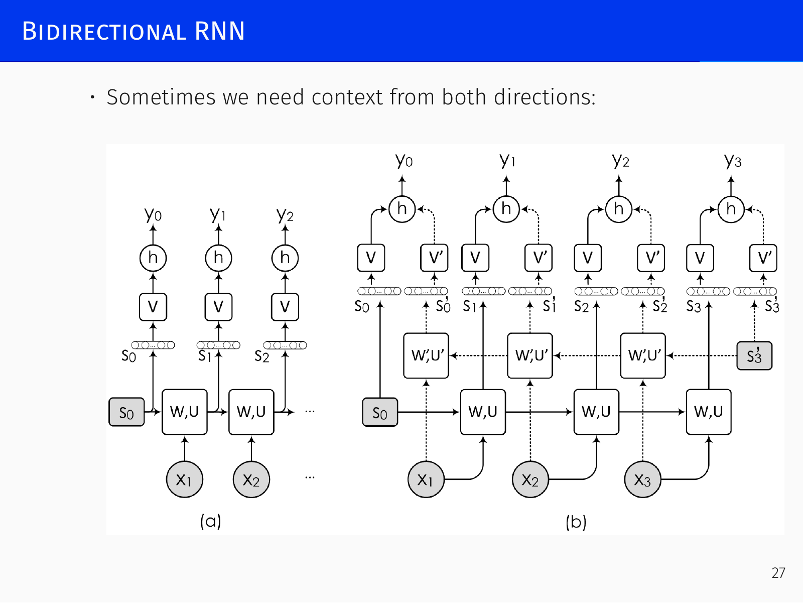
Unless the problem prohibits it (e.g., language modelling requires predicting the next word using only left context; real‑time tracking can look only a few frames ahead), bidirectional RNNs are standard and this principle generalises to any recurrent architecture.

LSTM and GRU

Vanishing gradients occur because the gradient must repeatedly pass through multiplication by $W$. To preserve long‑term memory, a shortcut for gradients – analogous to the skip connections in ResNet – is needed. This is called the constant error carousel.

LSTM (Long Short‑Term Memory)

LSTM (Hochreiter & Schmidhuber, 1995/1997; modern form by Gers & Schmidhuber, 2000) constructs a complex unit that explicitly controls memory. The LSTM cell maintains a cell state $c_t$ and a hidden state $h_t$. Gates control information flow.

Vanilla LSTM equations:

• Candidate cell state: $c'_t = \tanh(W_{xc} x_t + W_{hc} h_{t-1} + b_{c'})$
• Input gate $i_t$: $i_t = \sigma(W_{xi} x_t + W_{hi} h_{t-1} + b_i)$
• Forget gate $f_t$: $f_t = \sigma(W_{xf} x_t + W_{hf} h_{t-1} + b_f)$
• Output gate $o_t$: $o_t = \sigma(W_{xo} x_t + W_{ho} h_{t-1} + b_o)$
• Cell state update: $c_t = f_t \odot c_{t-1} + i_t \odot c'_t$
• Hidden state: $h_t = o_t \odot \tanh(c_t)$

If the forget gate is fully open ($f_t = 1$), then $c_t = c_{t-1} + i_t \odot c'_t$ and $\frac{\partial c_t}{\partial c_{t-1}} = 1$ – the constant error carousel.

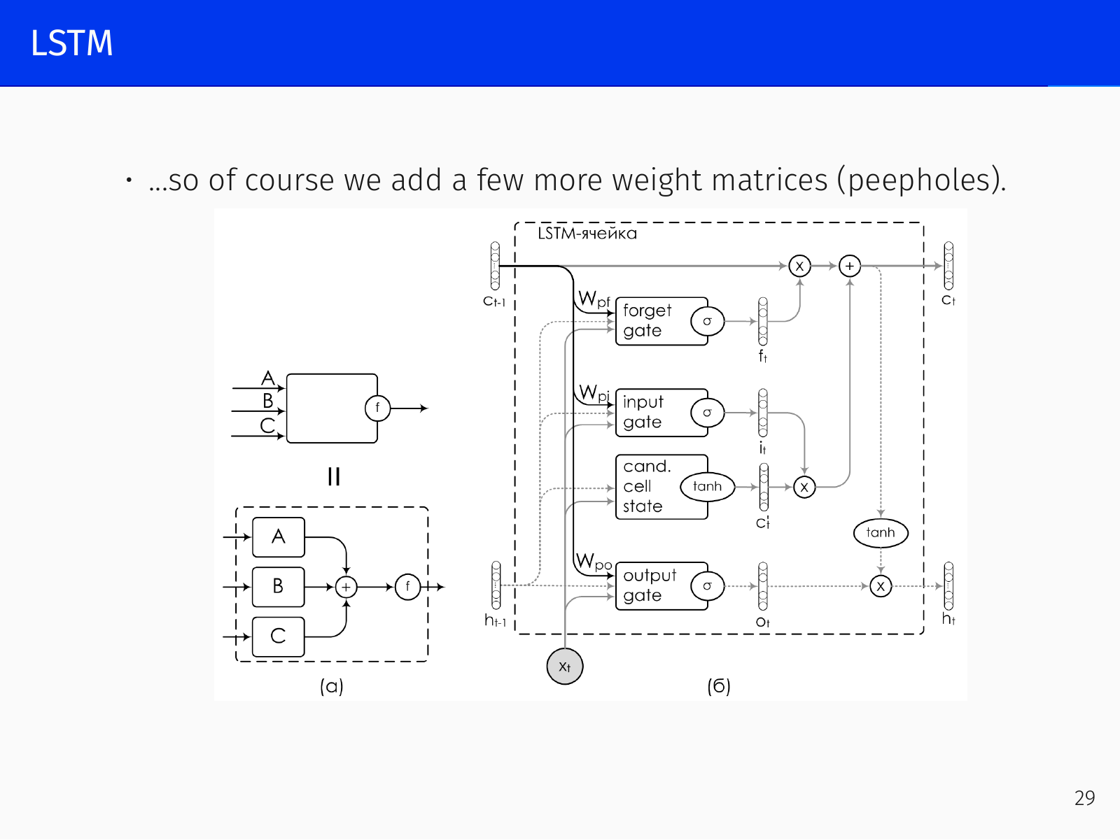
Peephole connections address the case where the output gate closes and the LSTM behaviour becomes independent of the cell state. They add the cell state directly to the gate computations:

Numerous LSTM variations exist; “LSTM: A Search Space Odyssey” (Greff et al., 2015) showed that some significantly simpler architectures (with one gate fewer) perform nearly as well.

GRU (Gated Recurrent Unit)

GRU (Cho et al., 2014) also implements the constant error carousel but with a simpler design. It merges the cell state and hidden state into a single state $h_t$ and uses only two gates:

• Update gate $u_t$: $u_t = \sigma(W_{xu} x_t + W_{hu} h_{t-1} + b_u)$
• Reset gate $r_t$: $r_t = \sigma(W_{xr} x_t + W_{hr} h_{t-1} + b_r)$
• Candidate hidden state: $h'_t = \tanh(W_{xh'} x_t + W_{hh'} (r_t \odot h_{t-1}))$
• Hidden state update: $h_t = (1 - u_t) \odot h'_t + u_t \odot h_{t-1}$

GRU uses 6 weight matrices (vs. 8 or 11 with peepholes) and fewer parameters, yet is only slightly worse than LSTM. Thus, under a fixed computational budget one can fit more GRU units, which often makes it competitive or even preferable.

Other variations exist; Józefowicz, Zaremba, and Sutskever (2015) performed a large evolutionary search over RNN architectures and identified several interesting alternative structures.