Vision Transformers and Object Detection

Vision Transformers 03:48

While Transformers were originally designed for sequences, they have been successfully adapted to images. The key insight is that an image can be treated as a sequence of patches, allowing a Transformer to process visual information without fundamental architectural changes. This section introduces several important architectures.

Visual BERT 03:48

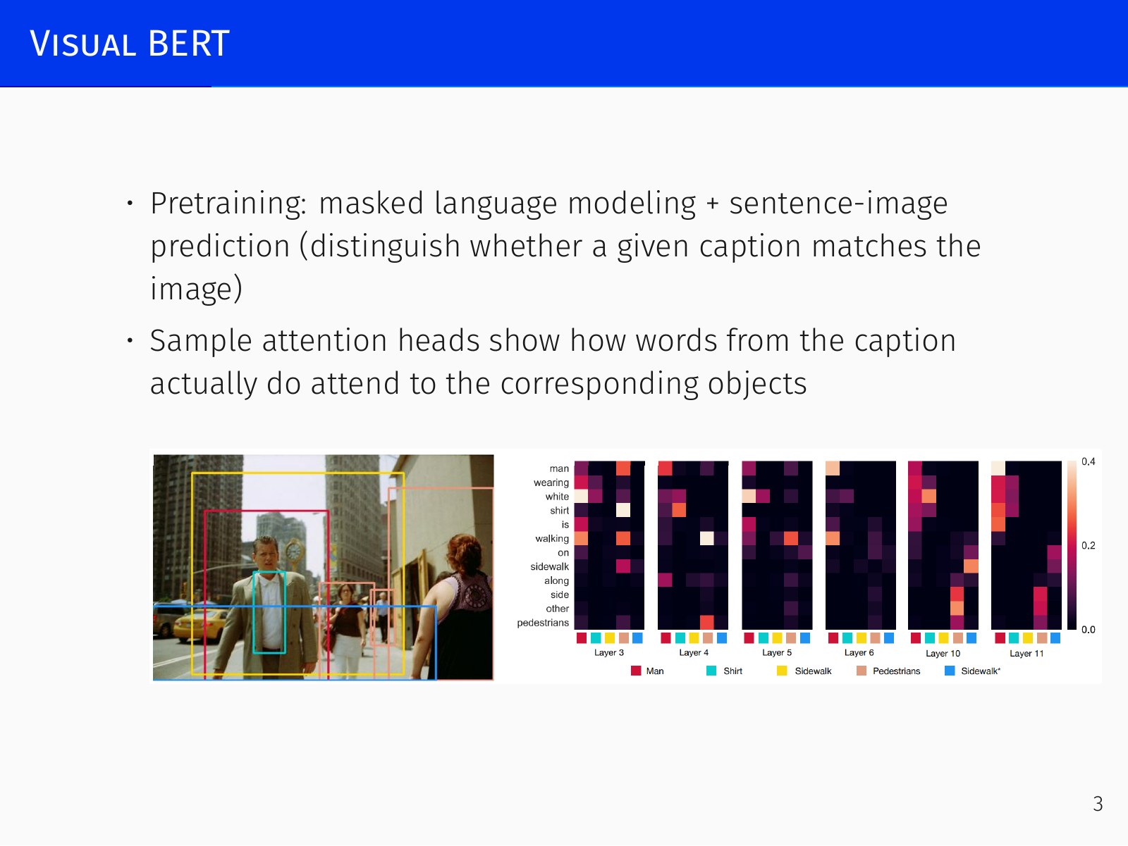
VisualBERT was one of the earliest attempts to jointly model images and text with a Transformer. It addresses tasks like image captioning by combining text tokens with object queries extracted from the image.

• The approach relies on a pretrained object detector (e.g., Faster R‑CNN) to crop out objects, embed them into vectors via CNNs with special positional embeddings, and feed them together with the caption words into a single Transformer.
• Pretraining uses masked language modeling and a sentence‑image prediction task (classifying whether a given caption matches the image). Attention heads show clear alignment between words and the corresponding visual objects.

Vision Transformer (ViT) 05:50

The Vision Transformer (ViT; Dosovitsky et al., 2020) applies the Transformer directly to images without any text input. Its simplicity is striking: it is essentially BERT but with image patches instead of word tokens, keeping the standard Transformer architecture entirely unchanged.

• An input image $x \in \mathbb{R}^{H \times W \times C}$ is cut into $P \times P$ patches, producing a sequence of $N = HW/P^2$ flattened tokens $x_p \in \mathbb{R}^{N \times P^2 \times C}$.
• Patches are linearly projected to embeddings and concatenated with a learnable [class] token; positional encodings (the same absolute encodings as in the original Transformer) are added.
• The sequence is fed into a standard Transformer encoder. Pretraining is performed via masked patch modeling, analogous to masked language modeling: a random subset of patches is replaced with a learnable [mask] embedding and the model must reconstruct them.

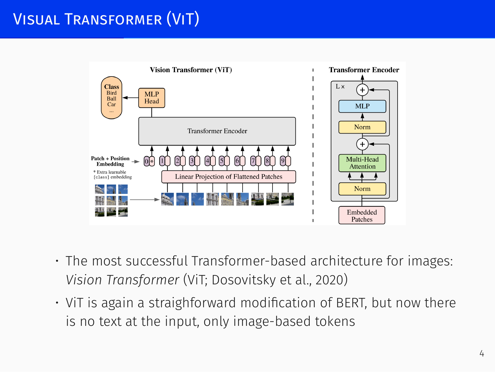
Despite the two‑dimensional structure of an image, experiments showed no benefit from using 2D positional encodings; simple sequence‑like encodings work just as well.

The ViT revolutionized computer vision because its self‑attention extracts semantically richer features than convolutional networks. In many applications, replacing a CNN backbone with a ViT backbone while keeping the top layers unchanged leads to immediate improvements.

Quadratic complexity and the patch‑size trade‑off

The main limitation of ViT is the quadratic complexity of self‑attention: the attention map is an $L \times L$ matrix, where $L = N$ is the number of patches. The number of patches grows as $(h/k)(w/k)$ for patch size $k \times k$, so handling high‑resolution details becomes infeasible. For example, a $1000 \times 1000$ image with $16 \times 16$ patches yields about $62 \times 62 \approx 3844$ tokens; the attention matrix has ~15 million entries, which is manageable, but with $4 \times 4$ patches we would have $250 \times 250 = 62500$ tokens and ~4 billion entries – quadratic blow‑up. Thus, ViTs are forced to use relatively large patches, losing fine details, which is especially problematic for detecting small objects. This trade‑off sparked research into hierarchical and window‑based transformers.

Swin Transformers 12:59

The Swin Transformer (Liu et al., 2021) addresses the quadratic cost by restricting self‑attention to local windows and building a hierarchical pyramid of features, similar to classical CNN backbones.

• The image is partitioned into a grid of non‑overlapping windows (e.g., $4 \times 4$ patches per window). Self‑attention is computed only within each window, reducing the complexity from $O(N^2)$ to $O(W^2)$, where $W$ is the window size, and the overall cost becomes linear in the number of patches.

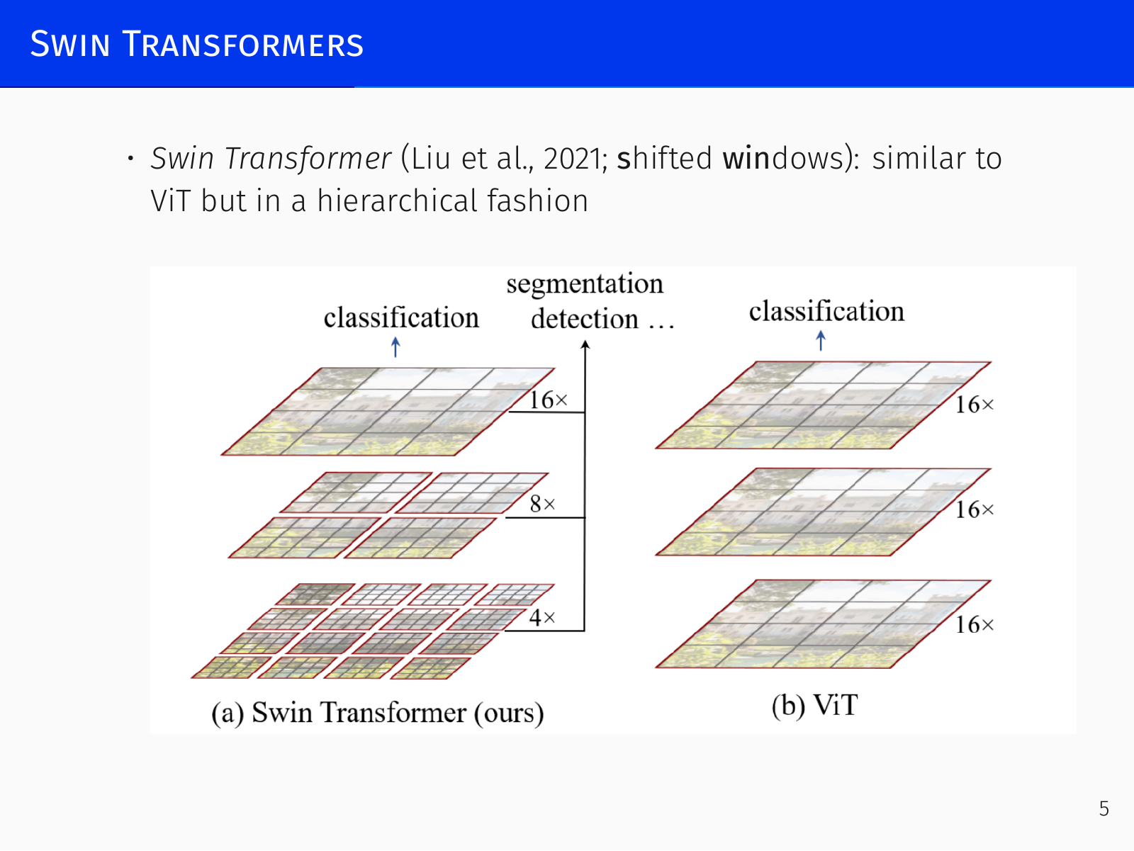
• Hierarchical processing: early stages work on small windows, later stages merge adjacent windows to form coarser feature maps, eventually producing a global representation. This multi‑scale structure allows the model to handle varying object sizes.
• Shifted windows: Between consecutive layers, the window grid is shifted by half the window size. Because each shifted window covers a different set of patches, this trick expands the receptive field without increasing computational cost. A patch that initially only sees a small region gradually aggregates context from a much larger area after a few layers.

This shifting creates a boundary problem: near image edges, the windows are no longer regular rectangles. The solution is to “roll” the image into a torus, pairing leftover edge pieces so that every window remains complete. While implementationally messy, this is only a minor edge effect and does not impact performance.

The Swin Transformer can scale to very large resolutions (up to $1536 \times 1536$ with Swin v2, 3 B parameters) and has become one of the most popular backbones for dense prediction tasks such as object detection and segmentation.

Perceiver

DeepMind’s Perceiver (Jaegle et al., 2021a) is a general‑purpose architecture that processes many modalities – images, point clouds, audio, video – without modality‑specific encoders.

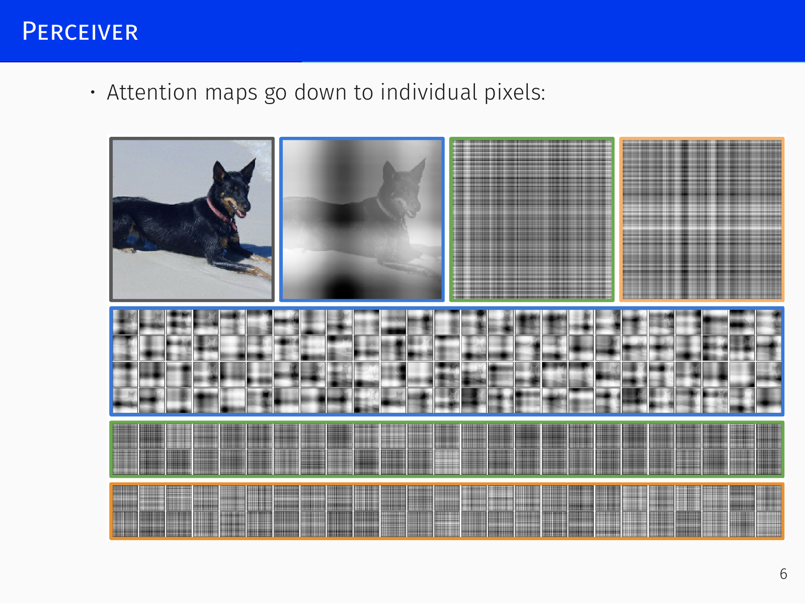
• To avoid the quadratic bottleneck, it uses a small set of latent vectors as queries that attend to a large array of input bytes (keys and values). This allows attention to operate at the level of individual pixels, even for high‑resolution inputs.

• Perceiver IO (Jaegle et al., 2021b) extends the architecture to produce high‑dimensional structured outputs, handling tasks such as optical flow, multi‑task language understanding, and StarCraft II. Output queries can be constructed using position coordinates and other properties, enabling the model to produce dense outputs.

Object Detection 23:27

Object detection is the task of identifying objects in an image and localizing them with bounding boxes. Unlike classification, which only produces a single class label per image, detection must handle a variable number of objects, each with a class label and four box coordinates.

Problem Setting 23:27

• A bounding box is defined by four numbers: typically the coordinates of one corner (e.g., bottom‑left) and the width and height. Thus each object output consists of a probability distribution over classes and a bounding box vector.
• The network must have a fixed number of outputs. Since we do not know in advance how many objects are present, we fix a maximal number of slots (say 100) and let each slot produce a confidence score (probability that an object exists), a class prediction, and a bounding box.
• At inference, we keep slots with high confidence and discard the rest.

Training: Loss Functions and Bipartite Matching 33:20

Training an object detector requires comparing the network’s fixed‑size set of predictions to the ground‑truth set of objects. Because objects have no natural order, we cannot simply align output slot $i$ with ground‑truth object $i$. Instead, we solve an assignment problem:

1. Pad the set of ground‑truth objects with “no object” ($\varnothing$) labels up to the fixed number of output slots $N$.
2. Find a one‑to‑one matching between the padded ground‑truth and the predictions that minimizes a total matching cost. This is a bipartite matching problem; the Hungarian algorithm provides the optimal permutation.
3. Once the matching $\sigma^*$ is determined, compute a training loss over the matched pairs.

The overall training loss typically has three components:

• Confidence loss: a binary cross‑entropy loss that encourages confidence to be 1 for slots matched to real objects and 0 for slots matched to $\varnothing$.
• Classification loss: cross‑entropy between the predicted class distribution and the true class, applied only to slots matched to a real object.
• Bounding box loss: measures the discrepancy between predicted and ground‑truth box coordinates, again only for matched objects.

Bounding box loss and IoU

A naive coordinate loss (e.g., L2 on $x, y, w, h$) treats large and small objects equally. For a large object, a moderate coordinate error still yields a decent overlap, while for a small object the same coordinate error can result in zero overlap – yet the numerical loss may be similar. To better reflect perceptual quality, modern detectors use the Intersection over Union (IoU):

IoU is differentiable when boxes overlap, providing meaningful gradients. However, when boxes are disjoint, IoU is 0 and its gradient vanishes, halting learning. Therefore, many detectors use Generalized IoU (GIoU), which extends the metric to non‑overlapping boxes and yields a gradient even when the intersection is zero.

R-CNN 52:01

The first successful deep‑learning‑based object detector was R‑CNN (Girshick et al., 2014). It works in stages:

1. An external algorithm, selective search, generates around 2000 class‑agnostic region proposals (bounding boxes that might contain an object).
2. Each proposed region is warped to a fixed size and fed through a CNN (pretrained on ImageNet, fine‑tuned on the detection dataset) to extract features.
3. An SVM classifies the features into object classes (or background), and a bounding box regressor refines the box coordinates.

R‑CNN won the ILSVRC 2013 detection challenge, but it was extremely slow – about 47 seconds per image on a GPU – because the full CNN forward pass had to be run for every proposal independently.

Fast R-CNN 59:59

Fast R‑CNN (Girshick, 2014) solves the speed problem by sharing computation:

• The whole image is passed through a CNN backbone once to obtain a high‑level feature map.
• For each region proposal, a small patch of the feature map is cropped via Region‑of‑Interest (RoI) projection (a non‑trainable geometric mapping).
• Because proposals have different sizes, each cropped feature region is pooled to a fixed size using RoI pooling: the region is divided into a fixed grid (e.g., $2 \times 2$) and max‑pooling is applied within each cell.
• A lightweight detection head (a small neural network) then classifies the pooled features and refines the bounding box.

This design is roughly two orders of magnitude faster than R‑CNN, with no loss of accuracy, but the proposals still come from the external selective search.

Faster R-CNN 1:06:35

The next bottleneck was the external proposal generator. Faster R‑CNN (Ren et al., 2015) integrates proposal generation into the network via a Region Proposal Network (RPN):

• The RPN operates on the same feature map from the backbone, sliding a small window and predicting, for each location, a set of predefined anchor boxes (boxes of various scales and aspect ratios) along with an “objectness” score and rough coordinates.
• The top‑scoring proposals (e.g., 300) are passed to the same RoI pooling + detection head pipeline as in Fast R‑CNN.

This makes the entire detector trainable end‑to‑end. Faster R‑CNN became the standard two‑stage detector for years, and its architecture exemplifies the modular separation between the backbone (feature extraction) and the detection head.

YOLO 1:13:03

YOLO (You Only Look Once; Redmon et al., 2016) takes a one‑stage approach, performing both box proposal and classification in a single forward pass:

• The image is divided into an $S \times S$ grid. Each grid cell predicts $B$ bounding boxes and class probabilities.

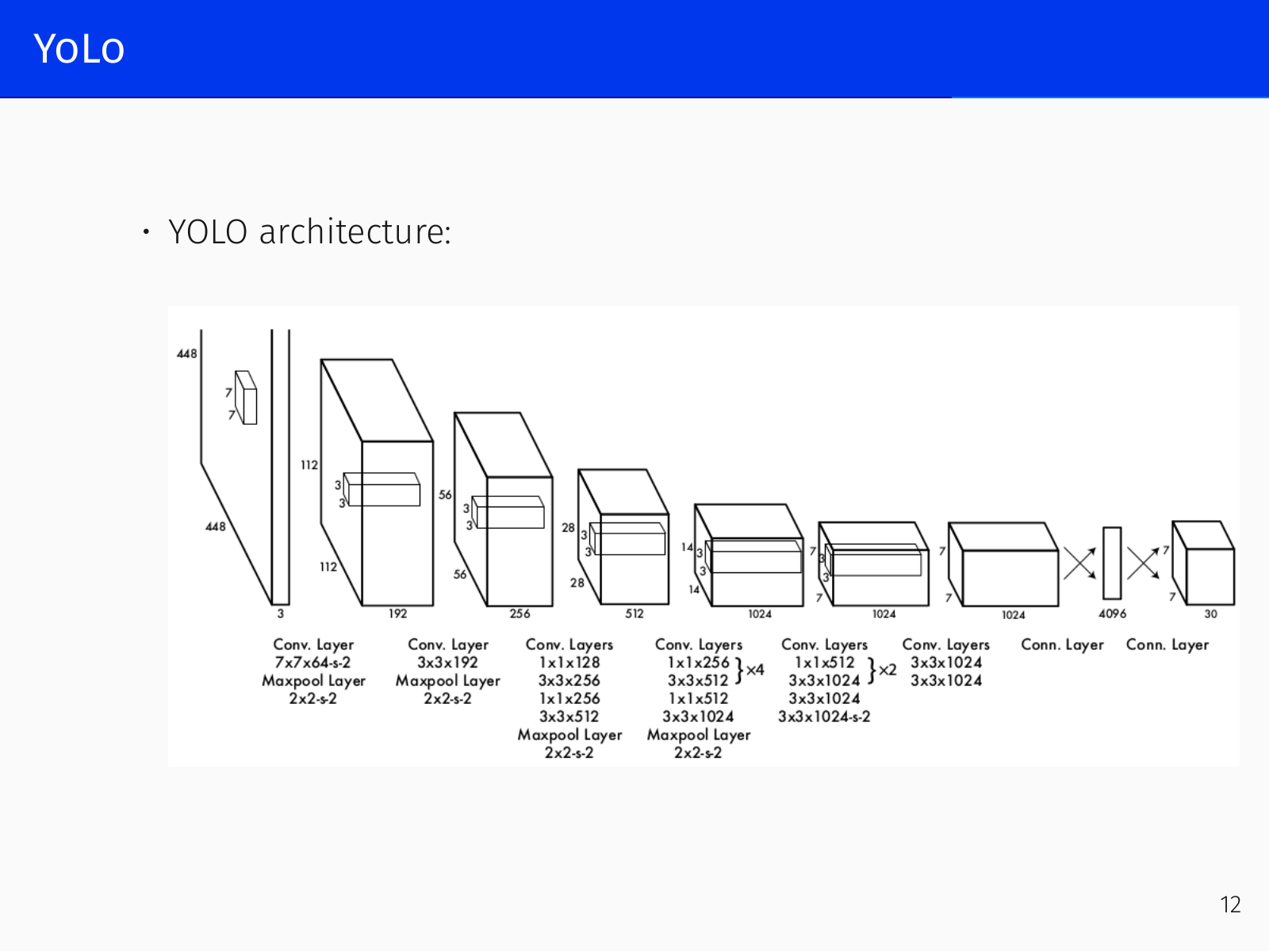
• The output is a tensor of shape $S \times S \times (5B + C)$, where each box has 5 components: $(x, y, w, h, \text{confidence})$, and $C$ class probabilities.
• The final score for a box containing a specific class is $p(\text{class}_i) \cdot \text{IoU}$ (originally $p(\text{class}_i \mid \text{obj}) \cdot p(\text{obj}) \cdot \text{IoU}_{\text{bbox}}$).
• Training is done with a single loss function where an indicator $\mathbb{1}_{\text{obj}}^{ij}$ specifies whether the $j$‑th box in cell $i$ is responsible for a given object.

YOLO is slightly less accurate than Faster R‑CNN but significantly faster and works out‑of‑the‑box. The YOLO family evolved through many versions (YOLOv2, YOLO9000, YOLOv3, etc.), accumulating small improvements that collectively yield large gains.

From Hand‑crafted Pipelines to Set Prediction 1:23:06

All classical detectors (R‑CNN, Faster R‑CNN, YOLO, SSD) rely on hand‑designed components: dense grids of anchor boxes, region proposals, and non‑maximum suppression (NMS) to eliminate duplicate detections. NMS is a non‑differentiable post‑processing step, and anchors require careful manual tuning. This motivated a fundamental question: Can we treat object detection as a direct set prediction problem, letting a Transformer predict the whole set of objects in one go, without anchors or NMS?

The answer is the DETR family.

Object Detection with Transformers 1:24:52

DETR 1:24:52

DETR (DEtection TRansformer; Carion et al., 2020) reformulates object detection as a set prediction task, using a Transformer encoder‑decoder and a bipartite matching loss to learn to predict a fixed‑size set of objects.

• A conventional CNN backbone (e.g., ResNet) extracts feature maps, which are flattened and combined with positional encodings. The resulting sequence is processed by a Transformer encoder.
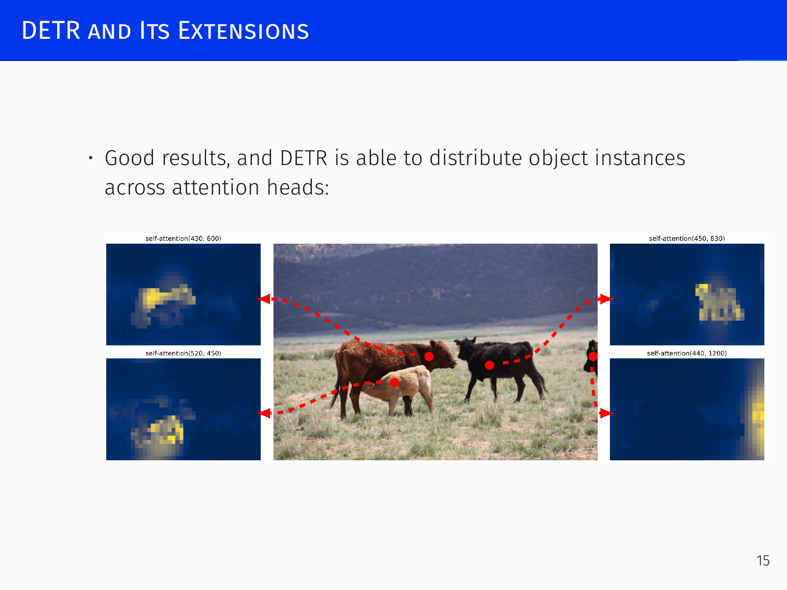
• The decoder receives a small fixed number of learnable object queries – vectors that act as input anchors and interact via self‑attention and cross‑attention with the encoder outputs. Each query eventually produces one detection (or a “no object”).
• A feed‑forward network on top of the decoder outputs class labels (including a special $\varnothing$ class) and bounding boxes.

Bipartite matching loss

The training relies on the Hungarian algorithm to find the optimal one‑to‑one matching between the $N$ predictions and the $N$ ground‑truth objects (padded with $\varnothing$):

The matching cost $\mathcal{L}_{\text{match}}$ is

where $\hat{p}_{\sigma(i)}(c_i)$ is the predicted class probability for the true class $c_i$, and $\ell_{\text{box}}$ combines $L_1$ and GIoU losses. The final training loss is

where “no object” predictions are down‑weighted by a factor (e.g., 0.1) to balance the loss.

Because the object queries interact via self‑attention in the decoder, they naturally avoid predicting the same object multiple times; no non‑maximum suppression is needed. Visualizations show that each query tends to specialise on a particular location, and decoder attention localises around object boundaries.

However, DETR operates on a single feature map scale, making it weak at detecting small objects. The global attention in the encoder also has quadratic complexity, limiting multi‑scale feature pyramids.

Deformable DETR 1:32:31

Deformable DETR (Zhu et al., 2021) introduces two key improvements:

• Multi‑scale feature maps: features from several layers of the backbone are used, enabling detection of objects at different sizes.
• Deformable attention: instead of attending to the entire feature map, each attention head learns to sample only a small, fixed number of points around a reference location. This reduces the complexity from $O(N^2)$ to linear in the number of tokens, making multi‑scale processing computationally feasible. The sampling offsets are learned jointly with the rest of the network.

DAB‑DETR 1:37:02

DAB‑DETR (Dynamic Anchor Box DETR; Liu et al., 2022) brings back the concept of anchor boxes, but makes them learnable and part of the query design. Each object query is parameterised as a bounding box $(x, y, w, h)$, which is gradually refined from decoder layer to layer. The width and height of the anchor box are used to modulate the cross‑attention, leading to better localised attention and much faster training convergence. This turns the abstract object queries into meaningful geometric entities from the start, helping the model separate queries across the image.

SMCA DETR

SMCA DETR (Spatially Modulated Co‑Attention; Gao et al., 2021) modulates the decoder’s cross‑attention weights by spatial priors: it biases attention towards locations close to predicted reference points, improving detection accuracy.

DN‑DETR

Early training stages of DETR suffer from unstable bipartite matching, where small changes in the network can cause completely different assignments. DN‑DETR (Li et al., 2022) stabilises training by adding a denoising objective: copy a subset of ground‑truth boxes, add noise to them, and feed them as additional “denoising queries” that must reconstruct the original boxes. This provides a strong anchor signal, helping the network learn accurate offsets.

DINO 1:37:02

DINO (Zhang et al., 2022) further improves DETR with several innovations, building on DN‑DETR:

• Negative examples: in addition to noisy ground‑truth boxes, it introduces anchors far from any object (large noise), forcing the model to learn to reject them. This strengthens the “no object” predictions.
• Mixed query selection: positional parts of object queries are initialised from region proposals generated by the encoder, while content parts remain learnable. This gives helpful location priors from the very first layer.
• Two‑step lookahead: DETR uses the current anchor box and predicted offset to update the box. DINO blocks gradient flow one additional step, updating layer $i$ parameters based on auxiliary losses from two consecutive predicted boxes ($b_i$ and $b_{i+1}$). This loosens the tight coupling between the anchor and offset and stabilises gradient propagation.

DINO achieves very strong results with fast convergence on a ResNet‑50 backbone, making it one of the top‑performing detectors at the time.

H‑Deformable‑DETR

Training DETR suffers from only a few positive matches per image. H‑Deformable‑DETR (Jia et al., 2023) simply duplicates positive queries: for each ground‑truth object, it adds extra queries that are also matched to the same object. Attention masks separate the different query groups to prevent them from interfering. This increases the number of positive examples and improves training efficiency.

UP‑DETR

UP‑DETR (Dai et al., 2021) introduces unsupervised pretraining for DETR. It randomly extracts patches from an image, and the model must predict the patch’s location and reconstruct its features – a task that encourages the encoder to build semantically meaningful representations, without needing classification labels.

DETReg

DETReg (Bar et al., 2022) replaces random crops with pseudo‑objects obtained from external algorithms (e.g., selective search, unsupervised region proposals) during self‑supervised pretraining. The model learns to predict embeddings for these regions, providing a better initialization.

Co‑DETR

Co‑DETR (Zong et al., 2023) attaches additional auxiliary detection heads from other object detection frameworks, which introduce new positive examples through their own matching procedures. This injects more training signal and improves the DETR‑style training.

Overview

The DETR family has evolved rapidly, as surveyed by Shehzadi et al. (2023). The core idea remains: a Transformer decoder processes a set of object queries to predict a set of objects, eliminating the need for hand‑designed anchor boxes and NMS. Subsequent works have focused on improving training stability, multi‑scale handling, query initialisation, and computational efficiency, resulting in state‑of‑the‑art detectors.