Convolutional Neural Networks

From Optimisation to Architecture 00:22

A neural network is a large computational graph composed of elementary operations. It receives two kinds of inputs: the actual data (e.g. an image) and the trainable weights. The graph’s final output is a scalar loss $L(x, y, w)$ , evaluated by comparing the prediction with the correct answer $y$ . The total loss over a mini‑batch $L(w)$ is the average of the per‑example losses. The weights are updated by gradient descent – or, in practice, by more sophisticated optimisers such as Adam:

w \leftarrow w - \eta\, \nabla_w L.

This simple loop (forward pass, loss, backward pass, weight update) captures deep learning in a nutshell.

When we design a network, we choose its architecture – the structure of the computational graph. The graph must be a directed acyclic graph (no cycles) so that it can be traversed topologically forward and backward. Every node must provide both a forward propagation and a backward propagation (gradient) computation.

A common organisation is the layered architecture. A layer is an informal set of neurons that mostly connect to neurons of the adjacent layers. Layers may be skipped by skip (residual) connections, which we will discuss later. The simplest class is the feed‑forward fully connected network: inside a layer, neurons do not connect to each other; each neuron receives inputs from all neurons of the previous layer and sends outputs to all neurons of the next layer – a complete bipartite graph between successive layers. Fully connected layers remain important and appear in modern architectures such as transformers.

Biological Inspiration: The Visual Cortex 09:35

Convolutional neural networks (CNNs) are one of the most influential architecture families. Their origin is partly biological, though the analogy eventually breaks down.

Why the brain does not run gradient descent

The human brain cannot perform gradient descent. A biological neuron possesses many dendrites and a single axon, so it can compute only one function – the forward pass. Gradient descent requires every node to compute two functions (forward and backward). Moreover, an error signal must somehow travel from the ultimate behavioural outcome back to every neuron. The brain does contain extensive feedback connections, but it certainly does not implement the precise gradient‑based credit assignment that artificial networks use. The architecture of the brain is fundamentally different: between every two layers there are feedback connections, and from later layers there are connections that reach all the way back, producing a tangled structure that we still do not understand in fine detail.

Hubel and Wiesel and the visual cortex

Visual cortex – the part of the cerebral cortex (occipital lobe) that processes visual information.

Hubel and Wiesel (Nobel Prize) pioneered single‑neuron recordings in the 1960s–70s. By attaching tiny electrodes to individual neurons in a live animal, they could read off which visual stimuli made each neuron fire.

They discovered an approximate hierarchical organisation:

V1 – local features (e.g. oriented lines, edges).
V2 – more local features, binocular vision.
V3 – colour, texture, first results of segmentation.
V4 – geometric shapes, silhouettes; crucial for attention.
V5 – motion of objects segmented in V4.
V6 – wide‑field stimulation; generalises data from the whole image; processes changes due to our own movement.
V7 (controversial) – recognition of complex objects, e.g. human faces.

Two broad processing streams emerge:

What pathway (V2 → V4): recognition of shapes and objects.
Where pathway (V2 → V5, V6): motion recognition, control over eyes and hands.

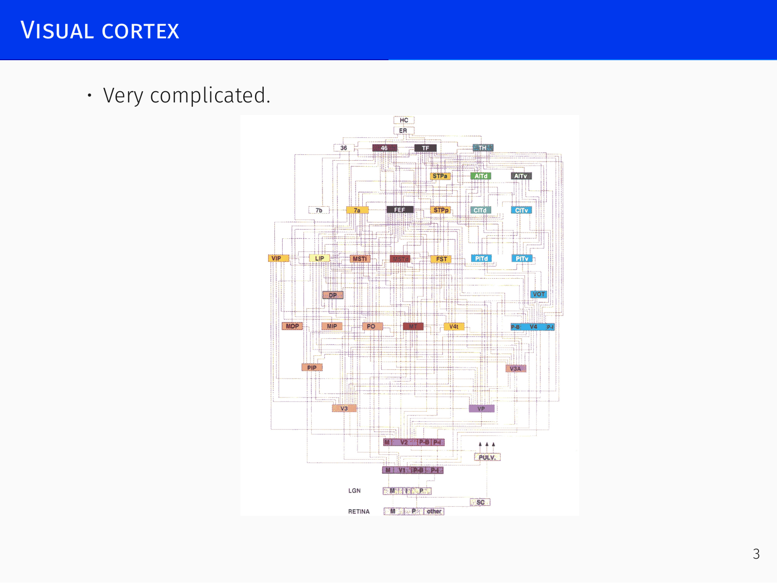
Visual cortex hierarchy and processing streams

Neurons in V1 have small receptive fields and respond to simple patterns – a vertical line, a horizontal line. Neurons in V2 combine them into more complex shapes (e.g. a corner). Beyond V2, the clean hierarchy dissolves into a dense mesh of feedback and lateral connections; there is no simple feed‑forward architecture like an artificial CNN.

From biology to the neocognitron

The observation that simple geometric shapes combine hierarchically, eventually enabling complex recognition, inspired attempts to mimic this in machines. The first such architecture was the neocognitron (Kunihiko Fukushima, 1979). It was a deep network with convolutional layers and hinge‑like activations (similar to ReLU), but it had no learning algorithm – the filters were hand‑crafted.

Trainable convolutional networks were created by Yann LeCun’s group in the late 1980s. They already appeared in essentially their modern form, with gradient‑based learning and convolution operations.

Convolutional Neural Networks: The Core Idea 25:59

The central assumption behind CNNs is a powerful structural regularisation: the operation we want to apply to the input is identical everywhere. If we have a detector that answers a question like “is there a face in this patch?”, then we apply exactly the same detector to every patch of the image. The inputs differ from patch to patch, so the answers differ, but the function is shared.

This leads to the following pipeline:

Break the input into (typically overlapping) windows.
An image is easiest to visualise, but the concept works for any data that can be tiled.
Apply a small neural network to every window.
This network has weights, is trained by gradient descent, and is extremely small because it sees only a local patch.
Construct a feature map – arrange the outputs of the small network in the same spatial order as the input windows. The result is a three‑dimensional tensor (width × height × feature depth).
Optionally compress the geometry with a pooling layer (usually max‑pooling).
Repeat – the output feature tensor can be fed into another convolutional layer, exactly as if it were a multi‑channel image.
Final prediction – after deep processing, pass the resulting feature tensor through one or more fully connected layers (a “classification head”) to produce the final output (e.g. class probabilities).

Because the small network is applied to every tile, its receptive field is very local. Stacking convolutions grows the receptive field only additively: a $3 \times 3$ convolution adds 2 pixels of context per layer. Looking at a $256 \times 256$ image would require about 130 layers – clearly impractical. This is the motivation for pooling layers.

Pooling: reducing geometry quickly 38:00

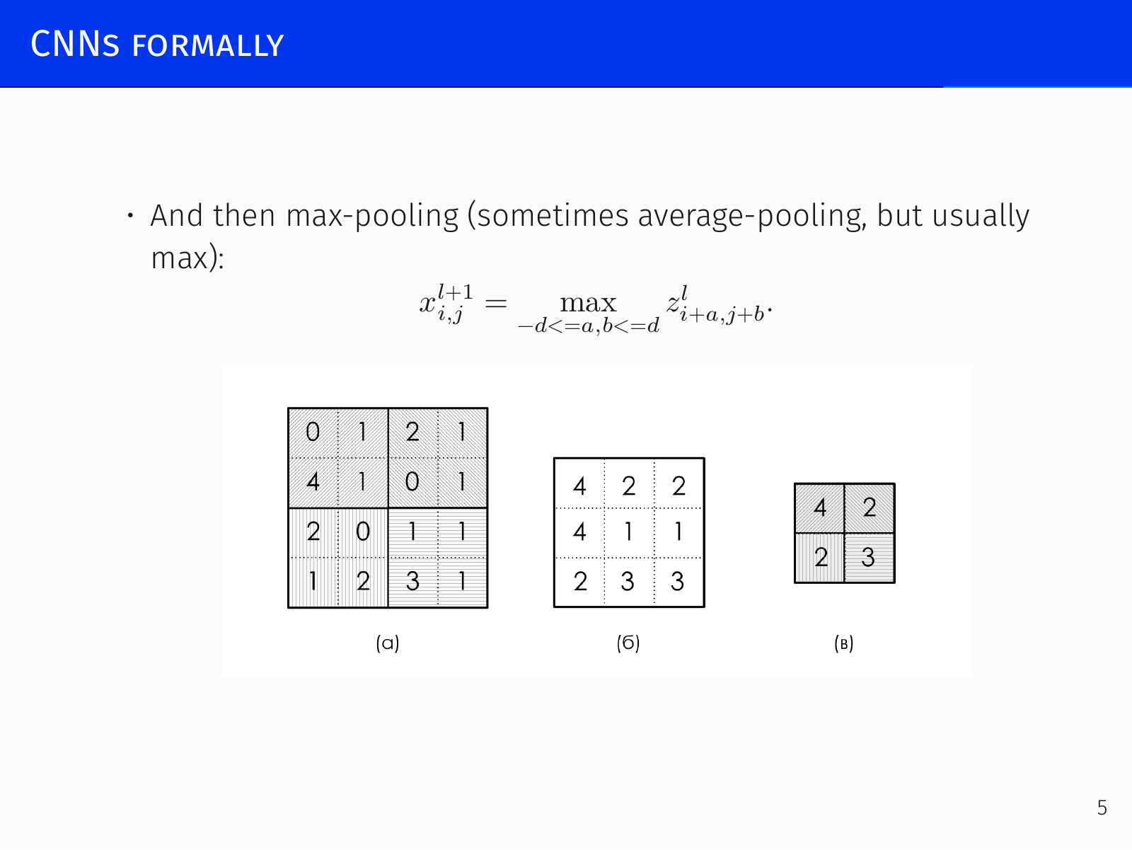
A pooling layer takes the feature map, slices it into non‑overlapping windows (typically $2 \times 2$ ), and replaces each window with a single value.

Max pooling – take the maximum.
Average pooling – take the average.

Max pooling is far more common in practice. Most features we care about in vision answer “is something present?”. If a head detector outputs $1$ for the correct patch and $0$ elsewhere, max pooling over a region yields $1$ wherever the head appears, while averaging would dilute the signal with all the zeros. Features that behave as presence detectors naturally compose via max, whereas features like average colour would be better served by averaging. Because convolutional networks are predominantly building shape detectors, max pooling is the default.

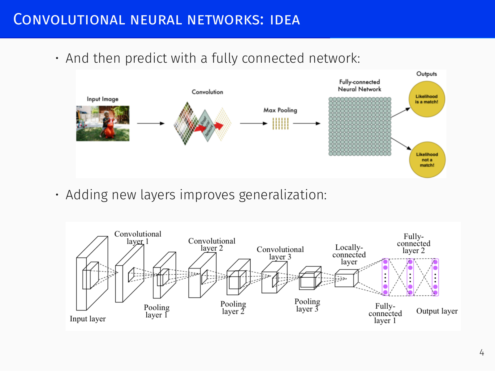
Max pooling operation over a feature map

With $2 \times 2$ pooling, each pooling layer halves the width and halves the height, reducing the number of values by a factor of four. Alternating convolution and pooling lets the network reach a large receptive field with far fewer layers.

CNNs Formally 43:04

Convolutional layer

A convolutional layer tiles the input with small windows and applies the same transformation to each window independently. When people say “convolutional layer”, they usually mean the simplest possible neural network inside each window: a single fully connected layer with shared weights.

Consider a three‑dimensional input of size $W \times H \times D$ (spatial width, height, feature depth; $D = 3$ for RGB, $D = 1$ for grayscale). We cut out a tile of size $w \times h \times D$ (always taking the full depth). This tile is flattened into a vector of length $D \!\cdot\! w \!\cdot\! h$ and multiplied by a weight matrix $\mathbf{W}$ of shape $(D w h) \times d'$ , producing an output vector of dimension $d'$ (the new “feature depth” for that location). The crucial property – weight sharing – is that exactly the same matrix $\mathbf{W}$ is reused for every tile of the input.

In practice, the weights are stored as a four‑dimensional tensor of shape $D \times w \times h \times d'$ (PyTorch convention). The input is a 3‑D tensor matching the first three dimensions, and the output is a feature map of depth $d'$ . The number of trainable parameters is $D \!\cdot\! w \!\cdot\! h \!\cdot\! d'$ , independent of the full input size.

The classical 2‑D convolution formulation is equivalent. Let $x^{(l)}$ be the feature map of layer $l$ . Using a square kernel of size $(2d+1) \times (2d+1)$ and weight matrix (kernel) $W$ , the linear part is

y^{(l)}_{i,j} = \sum_{-d \le a,b \le d} W_{a,b}\; x^{(l)}_{i+a,\,j+b}.

The notation emphasises that the same weights $W$ are applied at every position $(i,j)$ .

Convolution operation with shared weights

Nonlinearity

The result $y^{(l)}_{i,j}$ is then passed through a nonlinear activation $h$ . In modern CNNs this is almost always ReLU:

z^{(l)}_{i,j} = \max\!\bigl(0,\; y^{(l)}_{i,j}\bigr).

Because each weight is shared across all tiles, it appears many times in the computational graph. During backpropagation, the gradient for a weight is the sum of gradients across all those occurrences. The redundancy makes ReLU especially appropriate: zeroing out some activations still leaves plenty of signal from other tiles for the weight to learn.

Max pooling

A pooling layer with window size $(2d+1) \times (2d+1)$ operates on the activated feature map $z^{(l)}$ :

x^{(l+1)}_{i,j} = \max_{-d \le a,b \le d} z^{(l)}_{i+a,\; j+b}.

The windows are usually non‑overlapping; a $2 \times 2$ max‑pooling with stride 2 is the most common choice. Pooling layers contain no trainable parameters – they are deterministic functions.

Convolutions beyond 2‑D images 49:50

Convolutional layers are not limited to images. The same idea – cut the input into small tiles, apply a shared weight tensor – works for any domain that can be tiled:

1‑D convolution on sequences: Input is $L \times D$ (length × feature depth). A window of length $l$ slides along the sequence, flattening a $l \times D$ tile and multiplying by a shared weight tensor of shape $l \times D \times d'$ . The output is a vector of size $d'$ per position.
3‑D convolution on video: Input is $t \times w \times h \times D$ (time × width × height × depth). The weight tensor is five‑dimensional $t' \times w' \times h' \times D \times d'$ , and tiles are cut along all spatio‑temporal dimensions.

All examples in this lecture series will stay with images, where convolutions have been especially productive.

A Concrete Walkthrough: LeNet‑Style Architecture 52:45

To see the enormous savings in parameters, consider a small classical architecture inspired by LeNet (circa 2001).

Input – $32 \times 32$ grayscale image; tensor shape $1 \times 32 \times 32$ .

Layer 1 – convolution

Kernel size: $5 \times 5$ (implied by the fact that the output spatial size becomes $28 \times 28$ without padding, losing 4 pixels total).
Input depth $1$ , output depth (feature maps) $6$ .
Weight tensor: $1 \times 5 \times 5 \times 6$ .
Trainable weights: $5 \cdot 5 \cdot 6 = 150$ (ignoring biases).
Output tensor: $6 \times 28 \times 28$ .

A fully connected layer that maps the $32 \times 32$ input to a $6 \times 28 \times 28$ output would require a weight matrix of size $(32 \cdot 32) \times (6 \cdot 28 \cdot 28) = 1024 \times 4704$ , about 4.8 million parameters. The convolutional version uses only 150 – a massive compression of the hypothesis space. Weight sharing acts as an excellent structural regulariser.

Layer 2 – max pooling

Window $2 \times 2$ , non‑overlapping.
No trainable parameters.
Output: $6 \times 14 \times 14$ (each spatial dimension halved).

Layer 3 – convolution

Kernel $5 \times 5$ , input depth $6$ , output depth $16$ .
Weight tensor: $6 \times 5 \times 5 \times 16$ .
Trainable weights: $6 \cdot 25 \cdot 16 = 2400$ .
Output: $16 \times 10 \times 10$ (no padding, $14 \to 10$ ).

Layer 4 – max pooling

$2 \times 2$ pooling.
Output: $16 \times 5 \times 5$ .

Layer 5 – fully connected (classification head)

Now the spatial dimensions are only $5 \times 5$ . The whole tensor is treated as a single tile.

Input: $16 \times 5 \times 5 = 400$ values.
First fully connected layer: $400 \to 120$ neurons → $400 \cdot 120 = 48\,000$ weights.
Second fully connected layer: $120 \to 84$ neurons → $120 \cdot 84 = 10\,080$ weights.
Output layer: $84 \to 10$ neurons → $84 \cdot 10 = 840$ weights (plus softmax for classification).

Key observation: The total number of weights is roughly 60 000, of which the vast majority (about 57 000–58 000) reside in the final fully connected layers. The convolutional feature extractor contributes only around 2 500 weights. Convolutional layers do the heavy lifting of feature extraction while being extremely parameter‑efficient.

Padding and Stride 1:16:58

Padding

Applying a $K \times K$ convolution without any special treatment causes the spatial dimensions to shrink from $W \times H$ to $(W-K+1) \times (H-K+1)$ . To preserve the tensor shape across many layers, the input can be padded with extra values around the border before the convolution.

Zero padding – surround the image with zeros. This is simple but can create artificial edge responses because the kernel picks up many zeros near the boundary.
Mirror padding – reflect the edge pixels outward. This avoids introducing spurious zero‑valued features.

After padding, a $3 \times 3$ kernel can be centred on any original pixel, and the output retains the same spatial size.

Stride

Sliding the kernel over every possible position (stride 1) yields an output of almost the same size (with padding) or slightly reduced (without padding). To reduce the geometry more aggressively without pooling, one can use a stride larger than 1. For a stride of 2, the kernel is placed only on every second pixel in each direction, producing an output roughly $W/2 \times H/2$ . Every pixel is still covered (just fewer times), and no information is lost; the effective subsampling is built directly into the convolutional layer.

Formally, when defining a convolutional layer, we specify:

The weight tensor shape $D \times w \times h \times d'$ .
The padding (type and amount).
The stride – the step size in each spatial dimension (usually equal for both axes).

The trend in modern convolutional architectures (Inception, ResNet) has been to use pooling less often and to achieve geometric reduction through strided convolutions instead. Pooling can cut off computational paths and distort gradient flow; a strided convolution, although giving each pixel fewer processing steps, preserves a fully differentiable operation that is still a shared‑weight linear transform.